GSoC Report: Serialize Universes for parallel
31 Aug 2020As we approach the exascale barrier, researchers are handling increasingly large volumes of molecular dynamics (MD) data. Whilst MDAnalysis is a flexible and relatively fast framework for complex analysis tasks in MD simulations, implementing a parallel computing framework would play a pivotal role in accelerating the time to solution for such large datasets. In this Google Summer of Code project, we tried to touch on the basics to make sure the fundamental data structure of MDAnalysis—Universe can be serialized, and also streamlined the parallel framework.
Why and how do we serialize a Universe
A very short answer is: for multiprocessing. You know, processes don’t share memory in python. The pythonic way to share information between processes is called serialization—“Pickler” converts the objects into bytestream; “Unpickler” deciphers the bytestream into objects again. During serialization, states are conserved! But it does not sound as simple as it is; and of course, data structures as complex as Universe cannot be serialized easily. What we did in MDAnalysis, is taking the advantage of object composition in python and managing to serialize all the pieces and bits—topology and trajectory—that are crucial for reconstituting a parallel Universe.
One of the fundamental features of MDAnalysis is its ability to create a trajectory reader without loading the file into memory. It provides users with the ability not to ramp up their memory with huge trajectory files, but only loading the current frame into memory (and also random accessing all the frames). It is troublesome in the sense that the I/O Reader of python for such functionality is not picklable. One of the main achievements in PR #2723 is creating a pickling interface for all the trajectory readers.
Another key component of the Universe is its attached AtomGroup. Serializing AtomGroup before was error-prone. Users had to be super-cautious to first recreate/serialize a Universe then AtomGroup. Besides AtomGroup could not be serialized alone; when adding a reference from another Universe, it could only be the positions of the atoms but not AtomGroup itself. After the change in PR #2893, AtomGroup can be serialized alone; if it is pickled with its bound Universe, it will be bound to the same one after serialization; if multiple AtomGroup are serialized together, they will recognize if they are bound to the same Universe or not.
Finally, one of the coolest features that were introduced in version 0.19.0 is on-the-fly transformations (also as a previous GSoC project). You might wonder if you can perform a parallel analysis on a trajectory with the on-the-fly transformation present. Yes, you can…after PR #2859 is merged! You may want to find your favorite collective variables, and guide your further simulations, but most analysis has to be done on an ensemble of aligned trajectories. With the change, you can write a script to run the analysis directly on the supercomputer on-the-fly without jumping into the “trjconv hell”…and in parallel!
Okay enough technical terms talking. More information on serialization can be found in the online docs of MDAnalysis 2.0.0-dev; we also provide some notes on what a developer should do when a new format is implemented into MDAnalysis.
Parallelizing Analysis
So what’s possible now in MDAnalysis? Well you still cannot do analysis.run(n_cores=8) since the AnalysisBase API is too broad and we don’t really want to ruin your old scripts. What you can do now is use your favorite parallel tool freely (multiprocessing, joblib, dask, and etc.) on your personal analysis script. But before that, we should point out that per-frame parallel analysis normally won’t reach the best performance; all the attributes (AtomGroup, Universe, and etc) need to be pickled. This might even take more time than your lightweight analysis! Besides, e.g. in dask, a huge amount of time is needed overhead to build a comprehensive dask graph with thousands of tasks. The strategy we take here is called split-apply-combine fashion (Read more about this here Fan, 2019), in which we split the trajectory into multiple blocks, analysis is performed separately and in parallel on each block, then the results are gathered and combined. Let’s have a look.
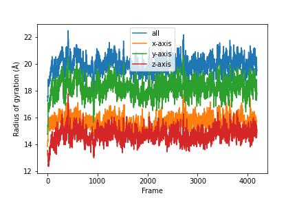
As an example, we will calculate the radius of gyration. It is defined as:
def radgyr(atomgroup, masses, total_mass=None):
    # coordinates change for each frame
    coordinates = atomgroup.positions
    center_of_mass = atomgroup.center_of_mass()

    # get squared distance from center
    ri_sq = (coordinates-center_of_mass)**2
    # sum the unweighted positions
    sq = np.sum(ri_sq, axis=1)
    sq_x = np.sum(ri_sq[:,[1,2]], axis=1) # sum over y and z
    sq_y = np.sum(ri_sq[:,[0,2]], axis=1) # sum over x and z
    sq_z = np.sum(ri_sq[:,[0,1]], axis=1) # sum over x and y

    # make into array
    sq_rs = np.array([sq, sq_x, sq_y, sq_z])

    # weight positions
    rog_sq = np.sum(masses*sq_rs, axis=1)/total_mass
    # square root and return
    return np.sqrt(rog_sq)
We will load the trajectory first.
u = mda.Universe(adk.topology, adk.trajectory)
protein = u.select_atoms('protein')
Split the trajectory.
n_frames = u.trajectory.n_frames
n_blocks = n_jobs   #  it can be any realistic value (0<n_blocks<=n_jobs, n_jobs<=n_cpus)

frame_per_block = n_frames // n_blocks
blocks = [range(i * frame_per_block, (i + 1) * frame_per_block) for i in range(n_blocks-1)]
blocks.append(range((n_blocks - 1) * frame_per_block, n_frames))
Apply the analysis per block.
A simple version of split-apply-combine code looks like this, it is decorated by dask.delayed, so it won’t be executed
immediately:
@dask.delayed
def analyze_block(blockslice, func, *args, **kwargs):
    result = []
    for ts in u.trajectory[blockslice.start:blockslice.stop]:
        A = func(*args, **kwargs)
        result.append(A)
    return result
We then create a dask job list; the computed results will be an ordered list.
jobs = []
for bs in blocks:
    jobs.append(analyze_block(bs, radgyr, protein, protein.masses, total_mass=np.sum(protein.masses)))
jobs = dask.delayed(jobs)

jobs.visualize()

results = jobs.compute()
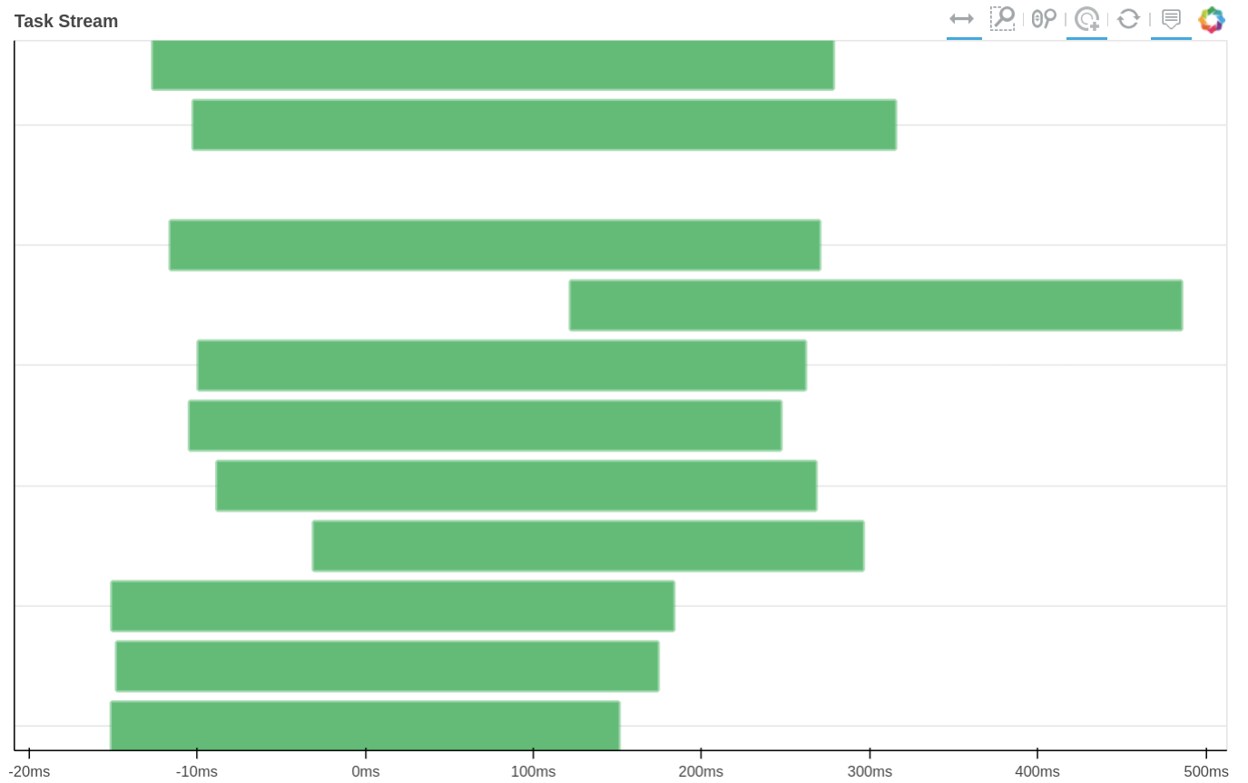
How tasks are divided can be visualized by jobs.visualize() and a detailed task stream can be viewed from dask dashboard—Each green bar here represents a block analysis job.


Combine the results.
result = np.concatenate(results)
result = np.asarray(result).T

labels = ['all', 'x-axis', 'y-axis', 'z-axis']
for col, label in zip(result, labels):
    plt.plot(col, label=label)
plt.legend()
plt.ylabel('Radius of gyration (Å)')
plt.xlabel('Frame')

A detailed UserGuide on how to parallelizing your analysis scripts can also be found here: User Guide: Parallelizing Analysis.
Future of parallel MDAnalysis
Of course, we don’t want to limit ourselves to some simple scripts. In Parallel MDAnalysis (PMDA), we are trying out what might be possible (PR #128, #132, #136 with this new feature to build a better parallel AnalysisBase API for the users. After PR #136, you will be able to use native features from dask to build complex analysis tasks and run multiple analyses in parallel as well:
u = mda.Universe(TPR, XTC)
ow = u.select_atoms("name OW")
D = pmda.density.DensityAnalysis(ow, delta=1.0)

# Option one (
D.run(n_blocks=2, n_jobs=2)

#  Option two
D.prepare(n_blocks=2)
D.compute(n_jobs=2)   #  or dask.compute(D)

#  furthermore
dask.compute(D_1, D_2, D_3, D_4...)  #  D_x as an individual analysis job.
Conclusions
These three months of GSoC project have been fun and fruitful. Thanks to all my mentors, @IAlibay, @fiona-naughton, @orbeckst, and @richardjgowers, (also @kain88-de and other developers) for their help, reviewing PRs, and providing great advice for this project. Now MDAnalysis has a more streamlined way to build parallel code for the trajectory analysis. What’s left to do is reaching a consensus on what the future parallel analysis API should look like, optimizing the dask worker footprint, reducing the time for the serialization process, and conducting conclusive benchmarks on different parallel engines.
Appendix
Benchmark
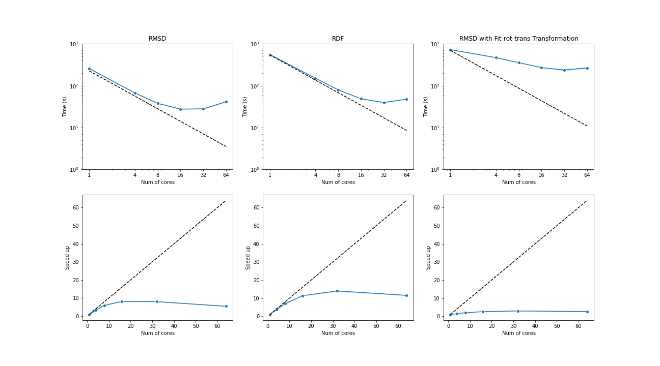
The benchmark below was run with four AMD Opteron 6274 (64 cores in total) on a single node. The test trajectories (9000 frames, 111815 atoms) were available at the YiiP Membrane Protein Equilibrium Dataset.
Three test cases were conducted under the latest MDAnalysis and PMDA code (PR #136)—RMSD analysis, a more compute-intensive RDF analysis, and the newly supported RMSD analysis with on-the-fly transformation (fit-rot-trans transformation in this case). All these cases show a strong scaling performance before 16 cores.

(Black dash line: ideal strong scaling performance; Blue: parallel performance (the number of blocks being splitted ie equal to the number of cores being used)
Major merged PRs
- #2723 Basic implementation of Universe and trajectory serialization. Tests and documents.
- #2815 Refactor ChainReader and make it picklable
- #2893 Make AtomGroup picklable
- #2911 Fix old serialization bugs to DCD and XDR formats