31 Aug 2020
As we approach the exascale barrier, researchers are handling increasingly large volumes of molecular dynamics (MD) data. Whilst MDAnalysis is a flexible and relatively fast framework for complex analysis tasks in MD simulations, implementing a parallel computing framework would play a pivotal role in accelerating the time to solution for such large datasets. In this Google Summer of Code project, we tried to touch on the basics to make sure the fundamental data structure of MDAnalysis—Universe can be serialized, and also streamlined the parallel framework.
Why and how do we serialize a Universe
A very short answer is: for multiprocessing. You know, processes don’t share memory in python. The pythonic way to share information between processes is called serialization—“Pickler” converts the objects into bytestream; “Unpickler” deciphers the bytestream into objects again. During serialization, states are conserved! But it does not sound as simple as it is; and of course, data structures as complex as Universe cannot be serialized easily. What we did in MDAnalysis, is taking the advantage of object composition in python and managing to serialize all the pieces and bits—topology and trajectory—that are crucial for reconstituting a parallel Universe.
One of the fundamental features of MDAnalysis is its ability to create a trajectory reader without loading the file into memory. It provides users with the ability not to ramp up their memory with huge trajectory files, but only loading the current frame into memory (and also random accessing all the frames). It is troublesome in the sense that the I/O Reader of python for such functionality is not picklable. One of the main achievements in PR #2723 is creating a pickling interface for all the trajectory readers.
Another key component of the Universe is its attached AtomGroup. Serializing AtomGroup before was error-prone. Users had to be super-cautious to first recreate/serialize a Universe then AtomGroup. Besides AtomGroup could not be serialized alone; when adding a reference from another Universe, it could only be the positions of the atoms but not AtomGroup itself. After the change in PR #2893, AtomGroup can be serialized alone; if it is pickled with its bound Universe, it will be bound to the same one after serialization; if multiple AtomGroup are serialized together, they will recognize if they are bound to the same Universe or not.
Finally, one of the coolest features that were introduced in version 0.19.0 is on-the-fly transformations (also as a previous GSoC project). You might wonder if you can perform a parallel analysis on a trajectory with the on-the-fly transformation present. Yes, you can…after PR #2859 is merged! You may want to find your favorite collective variables, and guide your further simulations, but most analysis has to be done on an ensemble of aligned trajectories. With the change, you can write a script to run the analysis directly on the supercomputer on-the-fly without jumping into the “trjconv hell”…and in parallel!
Okay enough technical terms talking. More information on serialization can be found in the online docs of MDAnalysis 2.0.0-dev; we also provide some notes on what a developer should do when a new format is implemented into MDAnalysis.
Parallelizing Analysis
So what’s possible now in MDAnalysis? Well you still cannot do analysis.run(n_cores=8) since the AnalysisBase API is too broad and we don’t really want to ruin your old scripts. What you can do now is use your favorite parallel tool freely (multiprocessing, joblib, dask, and etc.) on your personal analysis script. But before that, we should point out that per-frame parallel analysis normally won’t reach the best performance; all the attributes (AtomGroup, Universe, and etc) need to be pickled. This might even take more time than your lightweight analysis! Besides, e.g. in dask, a huge amount of time is needed overhead to build a comprehensive dask graph with thousands of tasks. The strategy we take here is called split-apply-combine fashion (Read more about this here Fan, 2019), in which we split the trajectory into multiple blocks, analysis is performed separately and in parallel on each block, then the results are gathered and combined. Let’s have a look.
As an example, we will calculate the radius of gyration. It is defined as:
def radgyr(atomgroup, masses, total_mass=None):
    # coordinates change for each frame
    coordinates = atomgroup.positions
    center_of_mass = atomgroup.center_of_mass()

    # get squared distance from center
    ri_sq = (coordinates-center_of_mass)**2
    # sum the unweighted positions
    sq = np.sum(ri_sq, axis=1)
    sq_x = np.sum(ri_sq[:,[1,2]], axis=1) # sum over y and z
    sq_y = np.sum(ri_sq[:,[0,2]], axis=1) # sum over x and z
    sq_z = np.sum(ri_sq[:,[0,1]], axis=1) # sum over x and y

    # make into array
    sq_rs = np.array([sq, sq_x, sq_y, sq_z])

    # weight positions
    rog_sq = np.sum(masses*sq_rs, axis=1)/total_mass
    # square root and return
    return np.sqrt(rog_sq)
We will load the trajectory first.
u = mda.Universe(adk.topology, adk.trajectory)
protein = u.select_atoms('protein')
Split the trajectory.
n_frames = u.trajectory.n_frames
n_blocks = n_jobs   #  it can be any realistic value (0<n_blocks<=n_jobs, n_jobs<=n_cpus)

frame_per_block = n_frames // n_blocks
blocks = [range(i * frame_per_block, (i + 1) * frame_per_block) for i in range(n_blocks-1)]
blocks.append(range((n_blocks - 1) * frame_per_block, n_frames))
Apply the analysis per block.
A simple version of split-apply-combine code looks like this, it is decorated by dask.delayed, so it won’t be executed
immediately:
@dask.delayed
def analyze_block(blockslice, func, *args, **kwargs):
    result = []
    for ts in u.trajectory[blockslice.start:blockslice.stop]:
        A = func(*args, **kwargs)
        result.append(A)
    return result
We then create a dask job list; the computed results will be an ordered list.
jobs = []
for bs in blocks:
jobs.append(analyze_block(bs, radgyr, protein, protein.masses, total_mass=np.sum(protein.masses)))
jobs = dask.delayed(jobs)
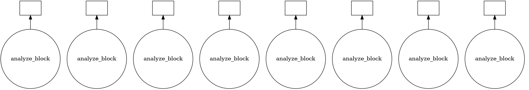
jobs.visualize()
results = jobs.compute()
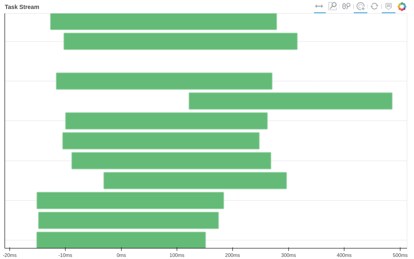
How tasks are divided can be visualized by jobs.visualize() and a detailed task stream can be viewed from dask dashboard—Each green bar here represents a block analysis job.
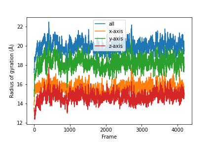
Combine the results.
result = np.concatenate(results)
result = np.asarray(result).T

labels = ['all', 'x-axis', 'y-axis', 'z-axis']
for col, label in zip(result, labels):
    plt.plot(col, label=label)
plt.legend()
plt.ylabel('Radius of gyration (Å)')
plt.xlabel('Frame')
A detailed UserGuide on how to parallelizing your analysis scripts can also be found here: User Guide: Parallelizing Analysis.
Future of parallel MDAnalysis
Of course, we don’t want to limit ourselves to some simple scripts. In Parallel MDAnalysis (PMDA), we are trying out what might be possible (PR #128, #132, #136 with this new feature to build a better parallel AnalysisBase API for the users. After PR #136, you will be able to use native features from dask to build complex analysis tasks and run multiple analyses in parallel as well:
u = mda.Universe(TPR, XTC)
ow = u.select_atoms("name OW")
D = pmda.density.DensityAnalysis(ow, delta=1.0)

# Option one (
D.run(n_blocks=2, n_jobs=2)

#  Option two
D.prepare(n_blocks=2)
D.compute(n_jobs=2)   #  or dask.compute(D)

#  furthermore
dask.compute(D_1, D_2, D_3, D_4...)  #  D_x as an individual analysis job.
Conclusions
These three months of GSoC project have been fun and fruitful. Thanks to all my mentors, @IAlibay, @fiona-naughton, @orbeckst, and @richardjgowers, (also @kain88-de and other developers) for their help, reviewing PRs, and providing great advice for this project. Now MDAnalysis has a more streamlined way to build parallel code for the trajectory analysis. What’s left to do is reaching a consensus on what the future parallel analysis API should look like, optimizing the dask worker footprint, reducing the time for the serialization process, and conducting conclusive benchmarks on different parallel engines.
Appendix
Benchmark
The benchmark below was run with four AMD Opteron 6274 (64 cores in total) on a single node. The test trajectories (9000 frames, 111815 atoms) were available at the YiiP Membrane Protein Equilibrium Dataset.
Three test cases were conducted under the latest MDAnalysis and PMDA code (PR #136)—RMSD analysis, a more compute-intensive RDF analysis, and the newly supported RMSD analysis with on-the-fly transformation (fit-rot-trans transformation in this case). All these cases show a strong scaling performance before 16 cores.
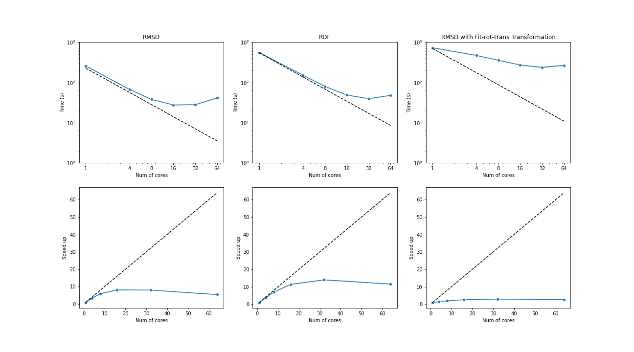
(Black dash line: ideal strong scaling performance; Blue: parallel performance (the number of blocks being splitted ie equal to the number of cores being used)
Major merged PRs
-
#2723
Basic implementation of Universe and trajectory serialization. Tests and documents.
-
#2815
Refactor ChainReader and make it picklable
-
#2893
Make AtomGroup picklable
-
#2911
Fix old serialization bugs to DCD and XDR formats
PRs to be merged
-
#2859
Serialization of transformations
-
#132
Refactor PMDA with the new picklable Universe
-
#136
New idea on how to refactor PMDA with dask.DaskMethodsMixin.
-
#102
UserGuide on how users can write their own parallel code.
— @yuxuanzhuang
29 Aug 2020
With the end of the summer comes the end of my awesome Google Summer of Code adventure with the MDAnalysis team. It’s also the occasion for me to report on the code I’ve implemented, the things I’ve learned and the challenges I’ve faced.
Summary of the project
The goal of my project, From RDKit to the Universe and back, was to provide interoperability between MDAnalysis and RDKit. i.e. to be able to:
- Read an RDKit Mol and create an MDAnalysis Universe with it,
- Convert an MDAnalysis AtomGroup to an RDKit Mol,
- Leverage RDKit’s functionalities directly from MDAnalysis (descriptors, fingerprints, aromaticity perception…etc.)
With this in mind, the project was easily cut down in 2 main deliverables (the RDKit Reader/Parser and the Converter) and a few smaller ones for each “wrapper” functionality.
The motivation behind the interoperability project was to be able to benefit from all the features that are available in RDKit and MDAnalysis with as little hassle as possible.
For example, before this project if you wanted to compute molecular descriptors for a ligand in an MD trajectory, you would have to write a separate PDB file for each frame of the trajectory and then read each file through RDKit. With the work that I’ve done, you can now convert your MD trajectory to an RDKit molecule and compute descriptors from there, or you can directly use the descriptor wrapper on an MDAnalysis AtomGroup (see below).
It was also the occasion for me to increase my visibility in the community by working on an open-source software development project, and to learn how to write better code. After my PhD I’d like to develop software for computational chemistry and this Google-sponsored event will hopefully help me in that regard.
Contributions
Merged PRs
-
Converting an RDKit molecule to MDAnalysis: #2707
This was the first part of the project and it helped me get acquainted with MDAnalysis as I had never used it before GSoC. The goal here was to be able to “parse” an RDKit molecule and build an MDAnalysis Universe from it.
It was also the occasion for me to start interfacing MDAnalysis with RDKit as I got to implement a new classmethod for the Universe, the Universe.from_smiles method which allows us to build a Universe from a SMILES string, but also to add atom selection based on aromaticity.
At the end of this first PR, I was familiar with the different core objects that compose the Universe as well as writing tests with pytest and documentation with sphinx.
-
Converting an MDAnalysis universe to RDKit: #2775
The second goal of the project was to be able to convert an MDAnalysis AtomGroup to an RDKit molecule, allowing users to analyse MD trajectories in RDKit. While this should be trivial once we know how to do the opposite operation, it was actually a real challenge to get a molecule with the correct bond order and charges out of it.
As you may know, most MD topology file formats don’t keep track of bond orders and formal charges so we have to find a way to infer this information from what we have. In our case, we require all hydrogen atoms to be explicit in the topology file, as well as elements and bonds (although these two can be guessed). Then the bond orders and formal charges are inferred based on atomic valencies and the number of unpaired electrons, followed by a standardization step of functional groups and conjugated systems. This last step is needed because the algorithm implemented to guess bond orders and charges is dependent on the order in which atoms are read.
Let’s take azathioprine as an example to visualize the different steps of the RDKitConverter:
 On the left is what you would get from a typical topology file: elements and bonds between atoms, but nothing more. In the middle, we’ve inferred bond orders and charges but because of the order in which atoms were read, two carbon atoms that were supposed to be part of the conjugated system end up negatively charged, and the nitro group isn’t represented in its usual form. On the right, we’ve corrected the purine ring and standardized the nitro group to obtain the final molecule.
This took more time than originally planned in the project timeline but was well worth it.
-
SMARTS selection: #2883
SMARTS is an extension of the SMILES language that is used for substructure searching. Being able to select atoms based on SMARTS queries, and combine these selections with those already available in MDAnalysis might be one of the key features that will come out of this project.
In progress
-
Wrap RDKit drawing code for AtomGroups: #2900
This PR allows us to draw images (SVG, PNG, and GIF) of AtomGroups using RDKit. It also adds rich displays to AtomGroups in notebooks (a.k.a. __repr__ methods).
Before working on this, I thought the only way to use alternative representations for Python objects was to define a _repr_*_ method for your class, where * is a MIME type such as png, html…etc. There is actually a second way, where you tell IPython directly how it’s supposed to represent an object. This allows funky representations of any object, even python built-in types, i.e. int as roman numerals and so on. I also wrote my first metaclass here, to register different “viewer” classes when more become available in the future. It’s also not straightforward to write tests for the images as different versions of RDKit or other packages will lead to slightly different outputs.
More discussion, code review, and tests are needed before this is ready.
-
Wrap RDKit descriptors and fingerprints: #2912
This PR adds new kinds of analysis that are typically performed on small molecules in the chemoinformatics field. Fingerprints are mostly used for calculating similarity metrics between molecules and a reference. Molecular descriptors could be used to describe all the sampled conformations of a ligand in a binding pocket during a simulation, and given as input to a machine-learning model for clustering, scoring binding poses…etc.
This is currently missing more discussion, documentation, and a few tests.
-
Change the Converters API: #2882
While developing the RDKitConverter, some interesting points were made about the current API used to convert AtomGroups, i.e. u.atoms.convert_to("RDKIT"). This method is case sensitive, it doesn’t allow to pass arguments to the converter class, and it requires users to read the documentation to know which converters are available. This PR corrects the two first points and adds the possibility to either use the previous syntax or tab-completion to find the available converters i.e. u.atoms.convert_to.rdkit().
This was inspired by pandas df.plot(kind="scatter", ...) which is also accessible as df.plot.scatter(...).
Since this is an API change, more discussion with core developers is needed for now.
Left to do
- Guessers for aromaticity and Gasteiger charges through RDKit
- Tutorial on the reader/converter and wrapped RDKit functionalities in the UserGuide. This will make it easier for users to know about the features I implemented and how to use them properly, rather than searching for every single feature in the documentation.
- Documentation on the RDKit format in the UserGuide: #69
Demo
Full circle
Here are all the possible conversions between RDKit and MDAnalysis:
import MDAnalysis as mda
from rdkit import Chem

# new feature
u1 = mda.Universe.from_smiles("CCO")
# new feature
mol1 = u1.atoms.convert_to("RDKIT")
# new feature
u2 = mda.Universe(mol1)
# before this project
u2.atoms.write("mol.pdb")
mol2 = Chem.MolFromPDBFile("mol.pdb")
Atom selections
There are two new selections available in MDAnalysis: aromatic for aromatic atoms, and smarts for the selection of atoms based on SMARTS queries. Let’s try them on this molecule:
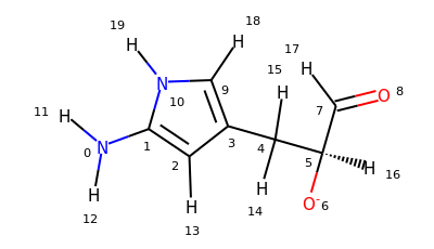
>>> u = mda.Universe.from_smiles("Nc1cc(C[C@H]([O-])C=O)c[nH]1")
>>> u
<Universe with 20 atoms>
>>> u.select_atoms("aromatic")
<AtomGroup with 5 atoms>
# same as above
>>> u.select_atoms("smarts a")
<AtomGroup with 5 atoms>
# 4 aromatic carbon atoms
>>> u.select_atoms("smarts c").indices
array([1, 2, 3, 9])
# carbon atoms in a ring (not necessarily aromatic)
>>> u.select_atoms("smarts [#6;R]").indices
array([1, 2, 3, 9])
# 1 aromatic nitrogen
>>> u.select_atoms("smarts n").indices
array([10])
# not hydrogen and not in a ring but connected to a ring
>>> u.select_atoms("smarts [$([!R][R])] and not type H").indices
array([0, 4])
Descriptors calculation
Soon, you will be able to compute descriptors directly from an AtomGroup, by either passing the name of the descriptor in RDKit, or by passing your own function that takes an RDKit molecule as argument.
Here’s an example of what the current version looks like:
>>> from MDAnalysis.analysis.RDKit import RDKitDescriptors
>>> u = mda.Universe.from_smiles("CCO", numConfs=3)
>>> def num_atoms(mol):
...    return mol.GetNumAtoms()
>>> desc = RDKitDescriptors(u.atoms, "MolWt", "RadiusOfGyration",
...                         num_atoms).run()
>>> desc.results
array([[46.06900000000002, 1.161278342193013, 9],
       [46.06900000000002, 1.175492972121405, 9],
       [46.06900000000002, 1.173230936577319, 9]],
      dtype=object)
Fingerprint calculation
You will also be able to obtain fingerprints:
>>> from MDAnalysis.analysis.RDKit import get_fingerprint
>>> fp = get_fingerprint(u.atoms, "AtomPair", hashed=True, nBits=1024)
>>> fp.GetNonzeroElements()
{36: 1,
 106: 1,
 297: 1,
 569: 3,
 619: 1,
 624: 8,
 634: 2,
 699: 1,
 745: 5,
 819: 4,
 938: 6,
 945: 3}
Drawing with RDKit
Finally, you will be able to display small AtomGroups as images in notebooks:
>>> from MDAnalysis.visualization.RDKit import RDKitDrawer
>>> from nglview.datafiles import PDB, XTC
>>> u = mda.Universe(PDB, XTC)
>>> elements = mda.topology.guessers.guess_types(u.atoms.names)
>>> u.add_TopologyAttr('elements', elements)
>>> u.atoms
<AtomGroup with 5547 atoms>
>>> ag = u.select_atoms("resname LRT")
>>> ag

You can also export any AtomGroup to a PNG or SVG, and even to a GIF for trajectories.
Conclusion
This project taught me a lot of things on software development and the Google Summer of Code experience has been incredible and valuable to me. All of this wouldn’t have been possible without the help of many people, including my amazing mentors (@IAlibay, @fiona-naughton and @richardjgowers), but also the rest of the MDAnalysis team as a lot of them got involved and gave me great feedback, so thank you to all of them!
— @cbouy
03 Aug 2020
On June 18 2020, MDAnalysis was pleased to release the first major version, 1.0.0. As described in our 2019 roadmap, this is the last version that supports 2.7. We will continue backporting relevant bug fixes where feasible (e.g. the upcoming 1.0.1), but the next major release will be 2.0.0, which will support Python 3.6+.
As we look forward to this next milestone, it is time to consider the next directions of MDAnalysis. The development of MDAnalysis has always been driven by the growing need for standardised, accessible analysis tools for open, reproducible, and collaborative research. While many major packages for molecular dynamics simulation provide their own set-up and analysis software, these are necessarily targeted to their own particular standards. MDAnalysis aims to provide analysis tools for simulation data in general, so historically a key objective has been to expand the number of supported package-specific data formats. As of version 1.0.0, we support over 40 file formats used in major packages for both molecular dynamics and quantum chemistry.
In 1.0.0 we also began to explore an exciting new approach: direct interoperability with other popular packages for molecular analysis by becoming API compatible instead of just file-format compatible, an approach also reinforced by discussions at the 2019 MolSSI Workshop: Molecular Dynamics Software Interoperability. Our new converters are distinct from topology parsers and coordinate readers as a third avenue for loading data into MDAnalysis. In 1.0.0 we added converters for two libraries: the molecular editor ParmEd, and chemfiles, a library for reading data from computational chemistry formats.
The general lack of interoperability between software packages in the molecular modelling community has been highlighted in the 2019 report of the NSF MolSSI on Molecular Dynamics Software Interoperability, noting consequences such as great duplication of effort in developing and maintaining similar tools across different formats; significant barriers to collaborating and transferring data; and requiring scientists to learn multiple packages and languages to access the full breadth of available analysis algorithms.
Moving forward, our plan is to increase the range of analyses and formats accessible to users by becoming interoperable with other relevant libraries. This reduces the need to duplicate and support existing tools within our own framework, and allows MDAnalysis to become a general-purpose analysis toolkit. We are already in the process of expanding compatible libraries in 2.0.0 by adding support for the widely popular RDKit cheminformatics toolkit through a Google Summer of Code projects
being carried out by Cédric Bouysset (@cbouy).
By the end of 2021, we aim to have expanded the range of our Converters framework to include packages in three categories: widely-used analysis libraries, such as MDTraj and pytraj; libraries that can expand the range of formats we can support, such as OpenBabel; and direct interfaces with computational chemistry engines such as OpenMM and Psi4.
Ensuring robust interoperability is best done as a community effort. If you are interested in contributing, or have comments or suggestions on our future directions, please get in touch!
— @MDAnalysis/coredevs