14 May 2024


MDAnalysis, in conjunction with the Molecular Sciences Software Institute
(MolSSI) and with the support of the Chan Zuckerberg Initiative and the
Center for Biological Physics, is holding a free, 2-day workshop on June
24th-25th 2024 at Arizona State University in Tempe, Arizona, USA.
This two-day workshop is intended to transform attendees from users to
developers and will cover an introduction to MDAnalysis, software best
practices, and guide participants through the creation of their own MDAKit.
This workshop is suitable for students and researchers in the broad area
of computational (bio)chemistry, materials science and chemical engineering. It
is designed for those who have familiarity with MDAnalysis and are
comfortable working with Python and Jupyter
Notebooks. For a better idea of things participants should be comfortable doing in Python or to freshen up on your skills, please have a look at the MolSSI lesson, “Python Scripting for Computational Molecular Science”. Workshop
participants should also already have a working conda or mamba installation of
MDAnalysis (mamba
preferred), as well as an editor of their choice for editing files.
Workshop Overview
MDAnalysis developers and experienced MolSSI instructors will teach
participants how to build their own MDAnalysis-based Python packages by guiding
them through the development of their own MDAKits. Specifically, the workshop
will include 3 modules: (1) an introduction to using and writing custom
analyses in MDAnalysis; (2) an overview of software development and maintenance
best practices; and (3) an interactive hackathon session where participants
write their own MDAKits.
The program will run from the morning of Monday, June 24th until the early
evening of Tuesday June 25th. Breakfast and lunch will be provided
together with tea/coffee during breaks.
Parts of the workshop will be held in a hybrid mode for those unable to attend
in-person. Registration for the hybrid components is required. Recordings of
hybrid sessions will be made available after the workshop.
Registration
Attendance at this workshop will be free but the in-person part of the
workshop will be limited to 40 participants. The workshop will be delivered to
a small group to allow interactive discussions, questions, and participant
engagement.
A number of bursaries will be available to assist with travel and
accommodation costs for participants from outside the greater Phoenix
area. Bursaries (up
to $600 in costs for US domestic travel) and up to 3 nights of hotel
accommodation (single room within 5 minutes of the workshop venue) will be
awarded and you can apply for them as part of the registration process.
Register by May 27, 2024 (midnight anywhere on Earth):
Register
Bursaries for in-person attendance
We especially welcome your application if you consider yourself being part of
an underrepresented demographic in the computational molecular sciences.
Bursaries are reserved to enable the attendance of participants from outside
the greater Phoenix area.
Note that airfare for travel awardees will have to be booked by June 3 through
our travel agency, so as an awardee you will have to be able to
respond to our communications (via email) immediately and act quickly.
Bursary recipients will be notified on May 29 or earlier.
Online participants
Part of the workshop will be taught in hybrid mode and if you are not able to
attend in person, please register for the online portion using the same
registration link above.
Travel
Tempe is part of the “Valley of the Sun” metropolitan area, which encompasses
Phoenix, the 5th most populous city in the US. Today the area is home to more
than 4.8 million people and encompasses the ancient lands of the Akimel O’odham
(Pima), Maricopa, and Tohono O’odham tribes.
Airport
Phoenix Sky Harbor PHX airport has direct connections to all major hubs
in the US.
PHX airport is 5.5 miles (10 minutes by car/rideshare) from the workshop venue.
Public transport (Light Rail)
The Valley Metro Light Rail connects the airport to Tempe along a
West-East axis. If your destination is near a Light Rail stop then
public transport works well:
- Take the free PHX Sky Train from the terminal to the 44th St/Washington
Metro Rail stop.
- Walk from the Sky Train stop to the Light Rail stop (all inside the 44th St
Sky Train structure)
- Buy a ticket at the ticket machine near the exit escalators to the Light
Rail stop.
- At the 44th St/Washington stop (Stop #10018) take the
east-bound Light Rail (direction Mesa, Gilbert Rd/Main St).
- The stop closest to the Hyatt Place Hotel and the workshop venue is
University Dr/Rural Rd (Stop #10023). If you want to get off closer to
downtown Tempe get off one stop earlier at Veterans Way/College Ave (Stop #10025)
- Walk to your destination.
Car/rideshare
To get from the airport to anywhere in Tempe either take a cab (traditional or self-driving
Waymo) or rideshare (Lyft, Uber).
Workshop Venue
The workshop will be held in the Student Success Center in the Department of
Physics at Arizona State University (room PSF 186 in the Physical Sciences F
building). The address is
Department of Physics
Arizona State University
Physical Sciences F Building
550 E Tyler Mall, PSF 186
Tempe, AZ 85287
USA
Paid parking is available in the Tyler Street Parking
Structure and other on-campus parking structures.
Accommodation
The closest hotel (5 min by foot) is the Hyatt Place Tempe.
Other hotels are available in Tempe within walking distance.
Weather
Arizona is hot during June. Temperatures in excess of 110ºF (43.3ºC) are not
rare, so it is important that you bring a hat/sunscreen for sun protection and carry
enough water with you.
Avoid hiking in the desert during the hot portion of the day (10am - 6pm), as it
can be deadly.
Workshop materials
All materials are made available in the https://github.com/MDAnalysis/MDAnalysisMolSSIWorkshop-Intermediate2Day repository.
If you have any questions or special requests related to this workshop, you may contact the organizing committee.
24 Apr 2024
MDAnalysis, in conjunction with MolSSI, is happy to announce an
upcoming in-person workshop, to be held June 24th-25th, 2024 at Arizona State University
(Tempe Campus). This two-day workshop is intended to transform attendees from users to developers
and will cover an introduction to MDAnalysis, software best practices, and guide participants
through the creation of their own MDAKit.
Attendance at this workshop will be free. A number of bursaries will be available to assist
with travel and accommodation costs. Places will be limited, but parts of the workshop will
be held in a hybrid mode for those unable to attend in-person.
Further details, including on the registration process, will be announced soon.
02 Apr 2024

MDAnalysis is applying for Google Season of Docs (GSoD) 2024. In this program, Google is sponsoring technical writers to work with open source projects in the area of documentation. Below is the project proposal we have submitted for this year’s program.
Consolidation and universal design of MDAnalysis resources for user learning
About your organization
MDAnalysis (current version 2.7.0, first released in January 2008) is an object-oriented Python library for temporal and structural analysis of molecular dynamics (MD) simulation data. MD simulations of biological molecules are an important tool for elucidating the relationship between molecular structure and physiological function. With thousands of users world-wide, MDAnalysis is one of the most popular packages for analyzing computer simulations of many-body systems at the molecular scale, spanning use cases from interactions of drugs with proteins to novel materials. As MDAnalysis can read and write simulation data in 30 coordinate file formats, it enables users to write portable code that is usable in virtually all biomolecular simulation communities. MDAnalysis forms the foundation of many other packages and is currently used by more than 20 data visualization, analysis, and molecular modeling tools. All MDAnalysis code and teaching materials are available under open source licenses, and the library itself is published under the GNU General Public License, version 3 or any later version (GPLv3+).
About your project
Your project’s problem
MDAnalysis is currently the most-used Python library for the analysis of simulation data in the molecular sciences due to its high-quality code base, extensive learning materials, and thorough documentation, but there is a considerable amount of overlap between our existing learning resources that makes it difficult for self-learners to find the information they need. Further, we seek to develop installation and training materials guided by Universal Design for Learning (UDL) principles to ensure accessibility of our learning resources. We therefore propose a reorganization and consolidation of the main website and additional MDAnalysis learning resources to guide diverse users through a streamlined workflow.
Consolidating learning resources to remove duplication
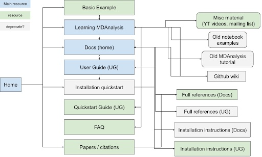
MDAnalysis’s participation in Google Season of Docs (GSoD) 2019-2020 was a quantum leap for our project, as a technical writer created the User Guide with the Quick Start Guide, which have become the primary entry points for new users. The GSoD work also catalyzed development of tutorial and online workshop materials. Although these materials are publicly available under open source licenses and are valuable resources for users, there is substantial overlap between MDAnalysis’s learning resources (main website, User Guide, docs, GitHub wiki) (Figure 1). Specifically, MDAnalysis resources (1) are duplicated across multiple hubs of information, (2) are organized such that new users stumble across developer-focused content early on, and (3) contain outdated tutorials and examples corresponding to older versions of the library.
 |
|
Figure 1: Map of current MDAnalysis learning resources and how they link to each other. Blue boxes indicate main hubs of material that also link to other resources, while green boxes correspond to simple resources. Resources inside gray boxes could be deprecated and their contents moved to other sites, if they are not already duplicated elsewhere. |
Universal design of installation training materials
We also expect that improving user experience with MDAnalysis learning resources will lower the barriers to adoption of MDAnalysis. MDAnalysis has run a number of workshops and created tutorials aimed at different audiences to get to know the package better. Materials include lecture slides and Python notebooks that demonstrate working code (e.g., materials from an online introductory workshop held in October 2023). This content provides a valuable resource to users – and much of it can be executed through Google Colab – but is most valuable to workshop participants and self-learners when they are able to set up a Python environment to run training materials on their own machines. MDAnalysis provides text-based installation instructions, makes workshop materials publicly available, and encourages workshop participants to inform us of measures we can take to lower barriers to their participation. Implementing universal design of additional audiovisual resources about installing and using MDAnalysis could make MDanalysis training materials more accessible to all, enhancing workshop participation and maximizing the asynchronous value of MDAnalysis’s learning resources.
Your project’s scope
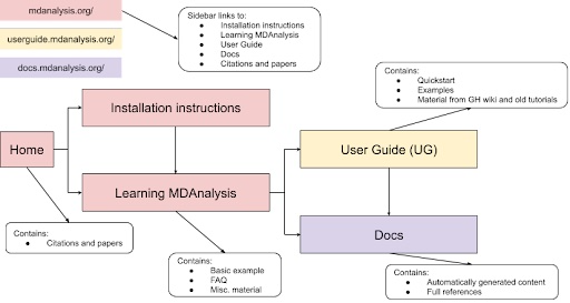
Through this project, we propose a cleanup of the main website and additional MDAnalysis learning resources to guide users through a streamlined workflow (Figure 2). The main body of each site (main website, User Guide, docs) would guide the user through the user process by limiting available choices and allowing quick jumping between the main hubs of information. In addition, this project will involve enhancing MDAnalysis learning resources following UDL guidelines.
 |
|
Figure 2: Proposed flow of MDAnalysis learning resources to ease user navigation. |
In particular, the MDAnalysis project will:
- Define the role of (and which content should be included in) the main website, User Guide, docs, and GitHub Wiki
- Merge the main website, User Guide, docs, and GitHub Wiki to de-duplicate information and guide users through the user process by incorporating quick jumping between the main hubs of information
- Identify and update any outdated material according to recent code releases, including removing old examples, outdated tutorials, and deadlinks and moving non-automatically generated content from docs into the User Guide
- Expand current tests for MDAnalysis notebooks and User Guide sections to more easily identify outdated materials in the future
- Integrate existing workshop materials and tutorials into the User Guide by pointing workshop materials to the User Guide where possible (e.g., descriptions of algorithms, units, etc.)
- Audit existing installation instructions/learning materials and revising and/or creating new materials according to UDL guidelines (e.g., developing audiovisual representations of installation across different operating systems, clarifying vocabulary used in tutorials, ensuring alt-text is included for visuals, etc.)
Measuring your project’s success
We will measure the success of our project according to the following metrics:
-
Reduced number of support requests. MDAnalysis core developers spend a considerable amount of time supporting users through our various communication channels, including our GitHub Discussions
forum, MDAnalysis
Discord Server, and our GitHub Issue Tracker. Many of these inquiries can be resolved by directing users to existing content on the main website, in the User Guide, or in the docs. The reorganization and accessibility audit of learning resources proposed in this project would provide users and self-learners with a faster and more efficient way to access relevant information.
-
Reduced number of docs-related issues on GitHub repository. We currently have 29 open docs-related issues on the MDAnalysis GitHub repository and another 47 issues on the User Guide repository. We anticipate the update, cleanup, and reorganization of our docs will close at least 5-10% of these outstanding issues (e.g., those related to duplication or outdated examples).
-
Increased number of visits to MDAnalysis learning resources. We regularly (and publicly) track web analytics for our main website using GoatCounter (currently nearly 50,000 unique visits per month). We will thus track whether the number of visits to the website, as well as to specific documentation (e.g., User Guide, tutorials, etc.), increase once our improved documentation is published. We aim to increase visits to current tutorials and learning resources by 30%.
-
Increased number of MDAnalysis installations and citations. A primary objective of this project is to enhance the user experience for newcomers to MDAnalysis and encourage continued growth in our user community. New releases are downloaded around 30,000 times per month (according to condastats and PyPI Stats over the last 12 months) and the academic papers describing MDAnalysis are cited over 3,500 times (Source: Google Scholar). A major milestone for this project will therefore be an increase in the number of new MDAnalysis installations per release. As a measure of sustained use of MDAnalysis, potentially indicating ease of use compared to similar packages in the academic community, we will monitor whether there is also an increase in the rate of MDAnalysis citations per year.
Timeline
We estimate that this work will take approximately 280 hours to complete. Once a technical writer is contracted, we will spend a month on tech writer orientation and identification of outdated material, then move onto the integration and updating of existing materials, as well as the enhancement of learning resources according to UDL guidelines. The contracted technical writer will have the flexibility to decide how to allocate the contract hours, either part-time or full-time, with the commitment to conclude the project within 6 months. The project timeline can be adapted to account for scheduling constraints of the hired writer.
| Dates |
Action Items |
| June |
Orientation, identify outdated material, and define the primary roles of the main website, User Guide, docs, and GitHub wiki. |
| July |
Integrate existing documentation from API docs into User Guide and remove duplication between main website, User Guide, and docs. |
| August |
Merge installation instructions from main website, User Guide, docs, and GitHub wiki. Remove old tutorials, old examples, and deadlinks, and expand tests to identify outdated material. |
| September |
Add links to point workshop materials and tutorials to the User Guide where possible. |
| October |
Audit existing installation instructions/learning materials and revise and/or create new materials according to UDL guidelines |
| November |
Continuation of ongoing work and project completion |
Project budget
The majority of the proposed budget is needed to support the substantial technical writer time required for this project. The project is set to affect multiple repositories and involves general restructuring of many resources, thus we anticipate a high level of involvement from the core developer team. Three MDAnalysis core developers – Dr. Micaela Matta (@micaela-matta), Prof. Oliver Beckstein (@orbeckst), and Dr. Lily Wang (@lilyminium) – and an emeritus core developer – Dr. Irfan Alibay (@IAlibay) – will be responsible for reviewing pull requests, assisting with site search and indexing tasks, mentoring the technical writer, and providing other necessary support to the GSoD program. The MDAnalysis program, community, and outreach manager, Dr. Jenna Swarthout Goddard (@jennaswa), will manage the logistics for recruiting the technical writer and will serve as the organization administrator for the GSoD program.
| Budget Item |
Amount |
Running Total |
Notes/Justification |
| Technical writer time |
$9,800 |
$9,800 |
280 hours (at a rate of $35/hour) |
| Mentor stipends |
$2,000 |
$11,800 |
4 volunteer stipends at $500 each |
| Swag |
$200 |
$12,000 |
T-shirts, stickers, etc. |
| TOTAL |
|
$12,000 |
|
Previous experience with technical writers or documentation
MDAnalysis previously worked with a technical writer through the GSoD 2019-2020 program. The technical writer, @lilyminium (MDAnalysis core developer since 2020), not only updated the User Guide, but also improved overall document appearance, fixed inconsistencies between materials, contributed code to the MDAnalysis library, and supported users. As @lilyminium was herself an MDAnalysis user, she was incredibly successful at independently generating new content and interacting with users to identify ongoing needs in the existing documentation. In addition, @pgbarletta has been working with the project since September 2022 on a NumFOCUS Small Development Grant aimed at improving and restructuring tutorial materials for future MDAnalysis workshops. As a newcomer to the project, he was quickly able to identify gaps and redundancies in the user guide and overall online documentation. His proposed improvements and modifications form the core of this GSoD proposal.
Previous participation in Google Season of Docs, Google Summer of Code or others
In addition to participation in GSoD 2019-2020 as described above, MDAnalysis has mentored 13 students through Google Summer of Code (GSoC) since 2016 (1-3 students annually) and 1 student through Outreachy 2022. Together, these initiatives have provided mentorship and support to early-stage open source developers, as well as encouraged progress on important issues and attracted long-term contributors. Several past GSoD, GSoC, and Outreachy participants are now core developers or ongoing contributors to the MDAnalysis library. In fact, 10 participants mentored through GSoD, GSoC, and Outreachy remain involved with the MDAnalysis project, with 4 of them serving as core developers and an additional 2 volunteering as mentors in this year’s GSoC program. Furthermore, MDAnalysis was awarded two Chan Zuckerberg Initiative (CZI) Essential Open Source Software for Science (EOSS) (rounds 4 and 5) grants. CZI EOSS4 has resulted in the establishment of the MDAKits, an ecosystem of downstream packages contributed by users of the main library. CZI EOSS5 enabled MDAnalysis to hire a dedicated project manager (Dr. Swarthout Goddard) to enhance the scope of MDAnalysis’s outreach, mentoring, and dissemination efforts. Dr. Swarthout Goddard will be providing administrative support throughout GSoD.